The parameters of pyqz

pyqz is designed to be easy and quick to use, but without withholding any information from the user. As such, all parameters of importance for deriving the estimates of LogQ and Tot[O]+12 can be modified via dedicated keywords. Here, we present some basic examples to clarify what does what. In addition to these examples, the documentation also contains a detailed list of the functions of pyqz, along with a brief description of each keyword.

First things first, let’s import pyqz and the Image module to display the figures.

%matplotlib inline
import pyqz
import pyqz.pyqz_plots as pyqzp

import numpy as np

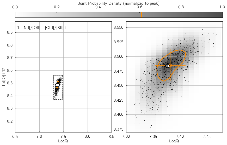
Parameter 1: srs

srs defines the size of the random sample of line fluxes generated by pyqz. This is an essential keyword to the propagation of observational errors associated with each line flux measurements. In other words, srs is the number of discrete estimates of the probability density function (in the {LogQ vs. Tot[O]+12} plane) associated with one diagnostic grid.

Hence, the joint probability function density function (combining \(n\) diagnostic grids) will be reconstructed via a Kernel Density Estimation routine from \(n\cdot\)srs points. srs=400 is the default value, suitable for error levels of $:raw-latex:sim`$5%. We suggest “srs=800` for errors at the 10%-15% level. Basically, larger errors result in wider probability density peaks, and thus require more srs points to be properly discretized - at the cost of additional computation time of course ! Try changing the value of my_srs in the example below, and watch the number of black dots vary accordingly in the KDE diagram.

my_srs = 800
pyqz.get_global_qz(np.array([[ 1.00e+00, 5.00e-02, 2.38e+00, 1.19e-01, 5.07e+00, 2.53e-01,
                               5.67e-01, 2.84e-02, 5.11e-01, 2.55e-02, 2.88e+00, 1.44e-01]]),
                   ['Hb','stdHb','[OIII]','std[OIII]','[OII]+','std[OII]+',
                    '[NII]','std[NII]','[SII]+','std[SII]+','Ha','stdHa'],
                   ['[NII]/[OII]+;[OIII]/[SII]+'],
                   ids = ['NGC_5678'],
                   srs = my_srs,
                   KDE_pickle_loc = './examples/',
                   KDE_method = 'multiv',
                   KDE_qz_sampling=201j,
                   struct='pp',
                   sampling=1)

# And use pyqz_plots.plot_global_qz() to display the result
import glob
fn = glob.glob('./examples/*NGC_5678*.pkl')

pyqzp.plot_global_qz(fn[0], show_plots = True, save_loc = './examples', do_all_diags = False)

--> Received 1 spectrum ...
--> Dealing with them one at a time ... be patient now !
    (no status update until I am done ...)

All done in 0:00:00.312550

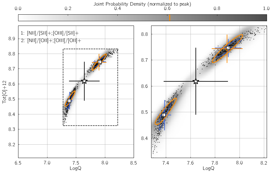
Parameter 2: KDE_method

This keyword specifies the Kernel Density Estimation routine used to reconstruct the individual and joint probability density functions in the {LogQ vs. Tot[O]+12} plane. It can be either gauss to use gaussian_kde from the scipy.stats module, or multiv to use KDEMultivariate from the statsmodels package.

The former option is 10-100x faster, but usually results in less accurate results if different diagnostic grids disagree. The underlying reason is that with gaussian_kde, the kernel bandwidth cannot be explicitly set individually for the LogQ and Tot[O]+12 directions, so that the function tends to over-smooth the distribution. KDEMultivariate should be preferred as the bandwidth of the kernel is set individually for both the LogQ and Tot[O]+12 directions using Scott’s rule, scaled by the standard deviation of the distribution along these directions.

In the example below, we insert some error in the [OII] line flux - thereby creating a mismatch between the different line ratio space estimates. Switch my_method from 'gauss' to 'multiv', and watch how the joint PDF (shown as shades of gray) traces the distribution of black dots in a significantly worse/better manner.

my_method = 'gauss'
pyqz.get_global_qz(np.array([[ 1.00e+00, 5.00e-02, 2.38e+00, 1.19e-01, 2.07e+00, 2.53e-01,
                               5.67e-01, 2.84e-02, 5.11e-01, 2.55e-02, 2.88e+00, 1.44e-01]]),
                   ['Hb','stdHb','[OIII]','std[OIII]','[OII]+','std[OII]+',
                    '[NII]','std[NII]','[SII]+','std[SII]+','Ha','stdHa'],
                   ['[NII]/[SII]+;[OIII]/[SII]+','[NII]/[OII]+;[OIII]/[OII]+'],
                   ids = ['NGC_09'],
                   srs = 400,
                   KDE_pickle_loc = './examples/',
                   KDE_method = my_method,
                   KDE_qz_sampling=201j,
                   struct='pp',
                   sampling=1)

# And use pyqz_plots.plot_global_qz() to display the result
import glob
fn = glob.glob('./examples/*NGC_09*%s*.pkl' % my_method)

pyqzp.plot_global_qz(fn[0], show_plots = True, save_loc = './examples', do_all_diags = False)

--> Received 1 spectrum ...
--> Dealing with them one at a time ... be patient now !
    (no status update until I am done ...)

All done in 0:00:00.561540

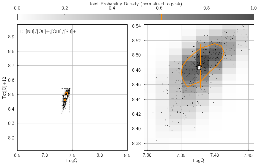
Parameter 3: KDE_qz_sampling

This sets the sampling of the {LogQ vs. Tot[O]+12} plane, when reconstructing the individual and global PDFs. Set to 101j by default (i.e. a grid with 101$:raw-latex:cdot\(101 = 10201 sampling nodes), datasets with small errors (\)<$5%) could benefit from using twice this resolution for better results (i.e. KDE_qz_sampling=201j). Resulting in a longer processing time of course. In the following example, the influence of KDE_qz_sampling can be seen in the size of the resolution elements of the joint PDF map, as well as the smoothness of the (orange) contour at 0.61%.

my_qz_sampling = 101j
pyqz.get_global_qz(np.array([[ 1.00e+00, 5.00e-02, 2.38e+00, 1.19e-01, 5.07e+00, 2.53e-01,
                               5.67e-01, 2.84e-02, 5.11e-01, 2.55e-02, 2.88e+00, 1.44e-01]]),
                   ['Hb','stdHb','[OIII]','std[OIII]','[OII]+','std[OII]+',
                    '[NII]','std[NII]','[SII]+','std[SII]+','Ha','stdHa'],
                   ['[NII]/[OII]+;[OIII]/[SII]+'],
                   ids = ['NGC_00'],
                   srs = 400,
                   KDE_pickle_loc = './examples/',
                   KDE_method = 'multiv',
                   KDE_qz_sampling=my_qz_sampling,
                   struct='pp',
                   sampling=1)

# And use pyqz_plots.plot_global_qz() to display the result
import glob
fn = glob.glob('./examples/*NGC_00*.pkl')

pyqzp.plot_global_qz(fn[0], show_plots = True, save_loc = './examples/', do_all_diags = False)

--> Received 1 spectrum ...
--> Dealing with them one at a time ... be patient now !
    (no status update until I am done ...)

All done in 0:00:00.120194

The other parameters

Most of the other parameters ought to be straightforward to understand (e.g. verbose). To use the maximum number of cpus available when running pyqz, set nproc = -1.

Check the page the functions of pyqz in the docs for more details.